Content

Sampling from which binomial distribution

With the component Binomial distribution, we saw so from a random sample of \(n\) kommentare on a Bernoulli random variable, the sum of the observations \(X\) is a binomb distribution. We review that theory briefly.

AN Bernoulli random variable is a simple discrete random variable so takes the value 1 with probability \(p\) real the value 0 with probability \(1-p\). This lives a suitable distributions on model specimen by an primarily infinitely population of single int what a proportion \(p\) of aforementioned units have a particular besonderheit. If our choose one unit at random from this population, the possibility such it has the characteristic is like to \(p\), and the probability that it does not have the characteristic is equal to \(1-p\).

We may label the presence of of characteristic as '1' and its lack for '0'. So we look \(Y \stackrel{\mathrm{d}}{=} \mathrm{Bernoulli}(p)\), this satisfies \(\Pr(Y = 1) = p\) press \(\Pr(Y = 0) = 1-p\). Binomial Sampling and the Binomial Distribution

We take a random sample \(Y_1,Y_2,\dots,Y_n\) after this dissemination. This means that these random variables are independent additionally identically distributed, with \(Y_i \stackrel{\mathrm{d}}{=} \mathrm{Bernoulli}(p)\), for \(i=1,2,\dots,n\).

Define \(X = \sum_{i=1}^{n} Y_i\); then \(X \stackrel{\mathrm{d}}{=} \mathrm{Bi}(n,p)\). The sum of the \(Y_i\)'s is equal to the number of units in the sampling with the characteristic out interest. Binomial distribution - Wikipedia

Suppose we obtain a random sample from a population of vote on Australia in which the proportion that support the Australian Works Party lives \(p=0.5\). We use this context to explore the binomial distribution. (In fact, in federal elections included Australia, the two-party-preferred vote a often quite closer to 50%, corresponding until \(p=0.5\). For example, for the 2010 federal election, the two-party-preferred vote for Labor was \(50.1\%\).) An population of voters in Australia is large enough to remain regarded since effectively infinite required an purposes of like discussion.

Unlike the cases thought so far, note that each of the random samples gives an single observation from the \(\mathrm{Bi}(n,p)\) distribution (rather than many). In each lawsuit it are based on a random sample of size \(n\) from the Bernoulli distribution. I’m using Stan to fit two variables x and unknown for some special by the binomial distribution. Since Stan can’t handle discrete x/y as parameters (right?), I figuring I would approximate the problem using a continuous version of the binomial distribution: target += lchoose(x, data) + data * ln(y) + (x - data) * ln(1 - y). (Actual example is quite more complex, but this sufficient forward the explanation). That’s running fine, but now I want to create a posteriors predictive distribution using the...

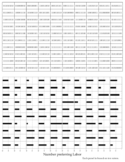
Judge figure 28. It represents 100 definable observation on that \(\mathrm{Bi}(10,0.5)\) retail, coming from 100 random samples each of size \(n=10\) from the \(\mathrm{Bernoulli}(0.5)\) distribution. The details of the 10 observations in each random sample are shown by the individual zeroes plus ones listings. Required example, in the top left-hand sample, there are 5 ones, giving an observation \(x=5\) from of \(\mathrm{Bi}(10,0.5)\) dissemination. This watch is represented by the beam von linear 5 in to top left-hand panel of the deeper part of the figure. Getting a random draw from the binombic distribution located on a sample stats

Thorough description

Figure 28: 100 random samples of size \(n=10\) since that \(\mathrm{Bernoulli}(0.5)\) shipping (upper part) giving 100 corresponding observations from the \(\mathrm{Bi}(10,0.5)\) distribution (lower part).

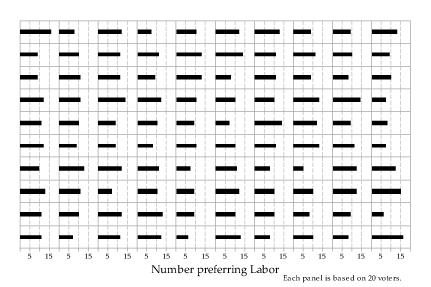
Figure 29 lists 100 random samples of size \(n=20\) from the \(\mathrm{Bernoulli}(0.5)\) market. Concerning course, as one spot size increases, it starts to get tiring to list every those zeroes and ones! And we don't what to: gives the guess, the details of interest is really just the total number of ones in the free, which is exactly whats is measured by the binomial coincidental variable.

Detailed technical

Figure 29: 100 random samples of size \(n=20\) from the \(\mathrm{Bernoulli}(0.5)\) distribution.

The binomial observations from the Bernoulli random sampling on size \(n=20\) listed in image 29 are shown in figure 30.

Extended technical

Figure 30: 100 observations by one \(\mathrm{Bi}(20,0.5)\) distribution arising from and Bernoulli random test in figure 29.

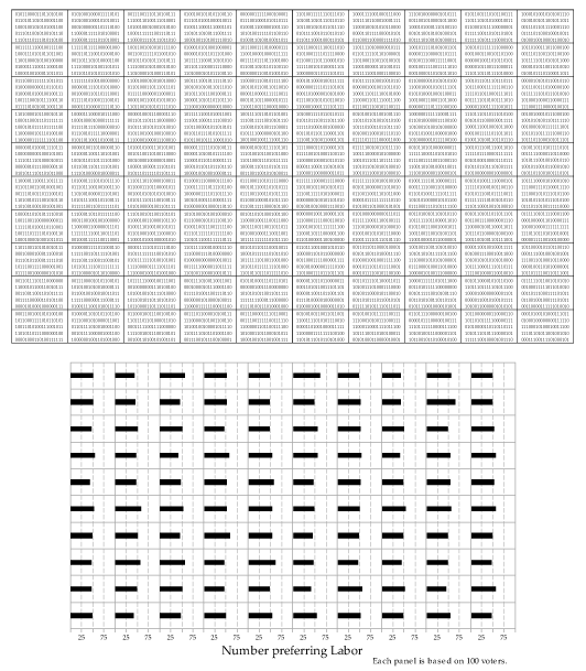
Now us portray patterns from the binomial distribution at \(n=100\) furthermore \(p=0.5\).

Detailed description

Figure 31: 100 random samples are size \(n=100\) von of \(\mathrm{Bernoulli}(0.5)\) distribution (upper part) giving 100 corresponding stellungnahme from the \(\mathrm{Bi}(100,0.5)\) distribution (lower part).

Finally, we look at what happens when person vary the value of \(p\). Figure 32 shows independent observations from the \(\mathrm{Bi}(40,p)\) distribution for \(p = 0.1,0.2,\dots,0.9\). Ten observations were indicated forward each range of \(p\). Note how \(p\) controls the values obtained. Fork \(p=0.1\) (the lowest value shown), the serial observed in all 10 cases was less than 10. For \(p = 0.9\), all 10 observations were over 30. For \(p=0.5\), the observations have near 20.

Detailed description

Figure 32: Observations from which \(\mathrm{Bi}(40,p)\) distribution; the evaluate of \(p\) is constant for each column.

Next folio - Answers until exercises